


The Big(O) Notation is a fundamental concept to help us measure the time complexity and space complexity of the algorithm. In other words, it helps us measure how performant and how much storage and computer resources an algorithm uses.
Also, in any coding interview, you will be required to know Big(O) notation. That will help you to get your dream job since every FAANG (Meta, Alphabet, Amazon, Apple, Netflix, Microsoft, Google) company will ask you that, even other companies.
The Big(O) notation is not 100% accurate, instead, it’s an estimate of how much time and space your algorithm will take. Another rule is that the Big(O) notation will be calculated considering the worst-case scenario.
Now that we have some understanding regarding Big(O) notation, let’s see the following diagram from the fastest O(1) to the slowest O(n!) time complexity:
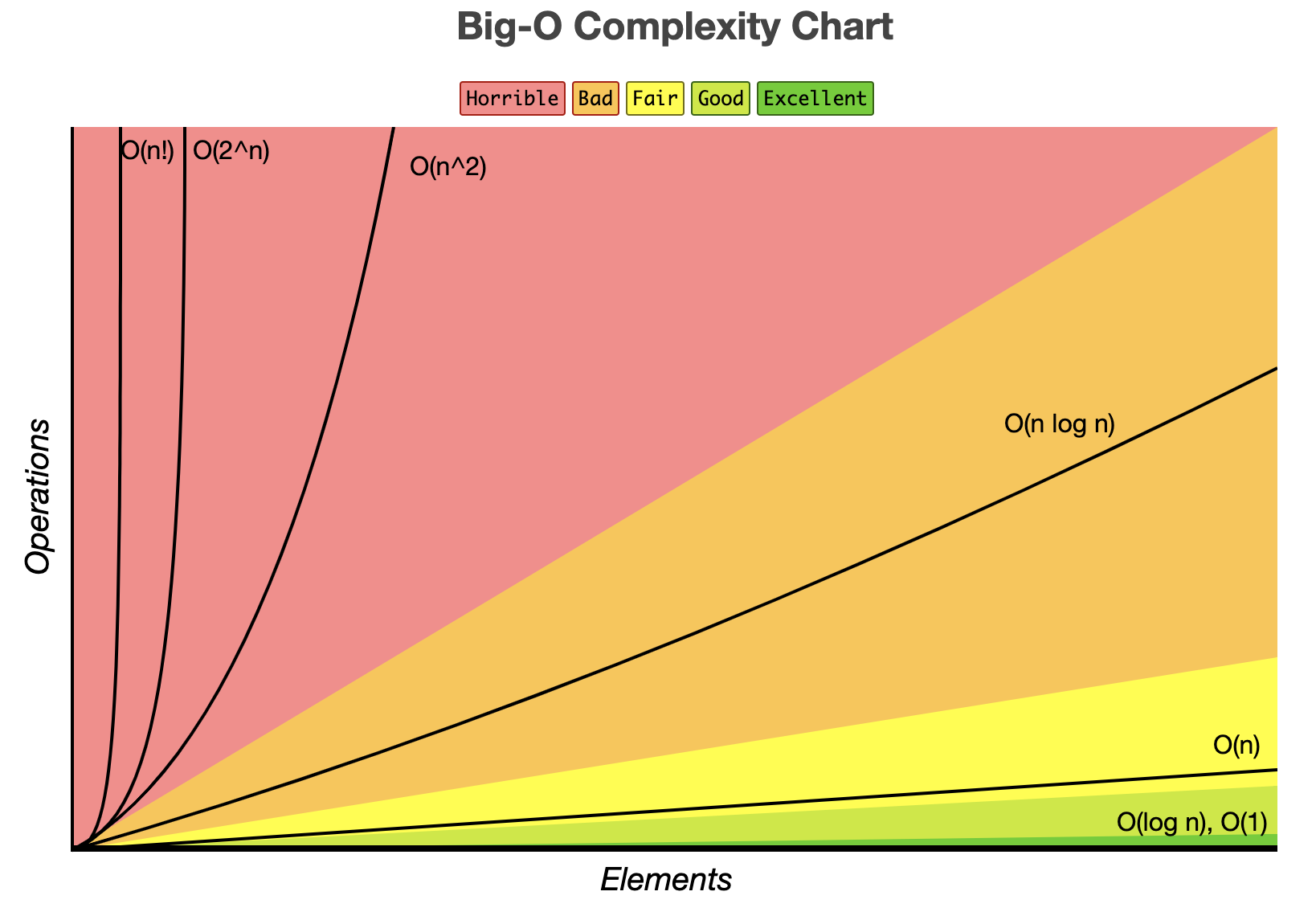
Source from https://www.bigocheatsheet.com
Asymptotic Notations
The asymptotic notation is a defined pattern to measure the performance and memory usage of an algorithm. Even though the Omega and Theta notations are not very much used in coding interviews, it’s important to know they exist.
Let’s see what are those asymptotic notations:
Omega Notation “Ω”: best-case scenario where the time complexity will be as optimal as possible based on the input. Theta Notation “Θ”: average-case scenario where the time complexity will be the average considering the input. Big-O Notation “O”: worst-case scenario and the most used in coding interviews. It’s the most important operator to learn because we can measure the worst-case scenario time complexity of an algorithm.
To see those notations in practice, let’s take the example of the Bubble sort algorithm:
The best-case scenario (Omega notation Ω) would be when the array is already sorted. In this case, it would be necessary to run through the array only once. Therefore the time complexity would be Ω(n).
The average-case scenario (Theta notation Θ) would be when the array has only a couple of elements unordered. In this case, it wouldn’t be necessary to run through the whole algorithm. Even though this is a bit better, the time complexity is still considered as O(n ^ 2).
The worst-case scenario (Big O notation) would be when the array is fully unsorted and the whole array has to be traversed. It would be necessary to sort the whole array, therefore, the time complexity would be O(n ^ 2).
The space complexity from the Bubble sort algorithm will be always O(1) since we only change values in place from an array. Changing values in place means that we don’t need to create a new array, we only change array values.
Constant – O(1)
In practice, we need to measure the Big(O) notation by checking the number of an elementary operation. In the case where we are creating an int number in memory, we are storing 8 bytes. If we were to be very precise with the Big(O) time complexity we would have to write O(8). But notice that this is a constant time. It doesn’t depend on any external number. It’s also irrelevant, O(8) doesn’t really change much performance. For this reason, we can consider that O(8) is actually O(1).
When assigning a variable this will take the time complexity of O(1) because it’s only one operation. Remember that the Big (O) notation will not measure precisely the performance of the algorithm. Therefore, the O(1) time complexity is an abstract way to measure code performance. Keep in mind that O(1) is pretty fast though. It’s doing only one light operation:
int number = 7; // O(1) time and space complexity
If we have a code with many operations and we are not using any kind of external parameter that will change the time complexity, it will still be considered as O(1). Let’s see the following code:
public class O1Example {

  public static void main(String[] args) {
    int num1 = 10;
    int num2 = 10;

    System.out.println(num1 + num2);
  }

}
Notice that even though the code above would be considered something around O(3), the number 3 is irrelevant because it doesn’t make much of a difference. Also, it doesn’t matter how many times we executed this algorithm it will have always a constant time complexity. Therefore, the code above also has O(1) of time complexity.
Also, notice that two values are being stored in two variables. Even though this is actually O(2) as space complexity, we can consider it as O(1) as well.
Accessing an Array by Index
Accessing an index of an array has also constant time complexity. That’s because once the array is created in memory, we won’t need to traverse the array, or do any other special operation. We just need to access it and the time complexity for that is O(1) or constant time:
int[] numbers = { 1, 2, 3};
System.out.println(numbers[1]); // O(1) here
Logarithmic – O(log n)
The classic algorithm that uses the O(log n) complexity is the binary search. That’s because it’s not necessary to run through the whole array. Instead, we get the number in the middle and check if it’s lower or greater than the number to be found. Then we break the array in two, we break it again until the number is found. That’s only possible because a binary search must have the array already sorted.
Let’s see the following diagram:
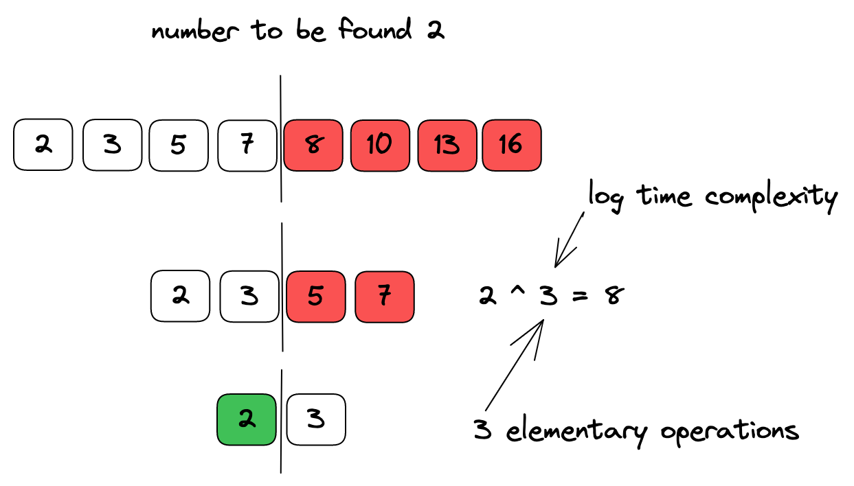
As you can see in the above diagram, instead of traversing the whole array we could break the array in two for three times and that was enough to find the number. That’s exactly the number we expect with the log complexity. That’s because 2 ^ 3 is the same as the size of our array. In other words, 2 2 2 = 8. Therefore, 3 is the log complexity of our number.
For you to notice how efficient and fast is the time complexity of log n, let’s think of an example. Suppose we pass an array from the size of 1048576 which is equivalent to 2 ^ 20, if you guessed that the number of iterations would be 20, you are right! In a linear complexity, the number of iterations would be 1048576 which is very slow.
Now that you understand better what is the log complexity, let’s see the code from the binary search algorithm:
Let’s see how is the code:
public class BinarySearch {

    public static int binarySearch(int[] array, int target) {
        int middle = array.length / 2;

        var leftPointer = 0;
        var rightPointer = array.length - 1;

        while (leftPointer <= rightPointer) {
            if (array[middle]  target) {
                rightPointer = middle - 1;
            } else {
                return middle;
            }

            middle = (leftPointer + rightPointer) / 2;
        }
        return -1;
    }

    @Test
    public void testCaseLog3() {
        int [] array = {2, 3, 5, 7, 8, 10, 13, 16};
        System.out.println(binarySearch(array, 2));
    }

    @Test
    public void testCaseLog20() {
        int [] array = new int[1048576];
        int number = 0;
        for (int i = 0; i < array.length; i++) {
            array[i] = ++number;
        }
        System.out.println(binarySearch(array, 1));
    }
}
Output: testCaseLog3: Iterations count: 3 0
testCaseLog20: Iterations count: 20 0
Another algorithm that has the time complexity of log(n) is the binary search tree. It’s similar to the binary search algorithm but has the difference that it will check numbers from a graph. If you are curious about this algorithm you can check the following link from javatpoint.
Linear – O(n)
When we use looping we have a linear complexity. It doesn’t matter if it’s the ‘for’, ‘while’, ‘foreach’, ‘do while’. Any of those loopings will have a linear complexity.
Let’s see a simple example:
public void printNumbers(int n) {
  for (int i = 0; i < n; i++) {
    System.out.println(i);
  }
}
Notice that the above code will print the number i that is incremented in each iteration. Since we run through the looping n times, we will have the time complexity of O(n).
Another important point is that if we have two loopings that depend on the same input, in our case, n we will still have the time complexity of O(n).
Let’s see how that translates in code:
  public static void printNumbers2Looping(int n) {
    for (int i = 0; i < n; i++) { // O(n)
      System.out.println(i);
    }

    for (int j = 0; j < n; j++) { // O(n)
      System.out.println(j);
    }
  }
As you can see in the above code, at first we might think that the time complexity is more than O(n) but it’s actually still O(n) because both loopings are using n as the size number.
Two Inputs – O(m + n)
To measure the time complexity we have to pay attention to the input numbers the algorithm is using. That will change the time complexity. If a looping depends on two inputs to be executed, the time complexity won’t be O(n), instead, it will be O(m + n) if we use two variables as the looping lenght.
Let’s see how that works in practice:
  public static void printNumbers(int m, int n) {
    for (int i = 0; i < m; i++) {
      System.out.println(i);
    }

    for (int i = 0; i < n; i++) {
      System.out.println(i);
    }
  }
As you can see in the above code, we have two inputs, m and n. Also, it doesn’t matter if the size of n is greater than m or vice-versa, the Big(O) notation will always be O(m + n) because m or n might be any number. Therefore, it might dramatically impact the time complexity of either m or n.
Log-linear – O(n log n)
Many efficient sorting algorithms such as Quicksort, Mergesort, and Heapsort have the time complexity of O(n log n). The time complexity O(n log n) is a bit slower than O(log n) and O(n).
The log-linear complexity is present in algorithms that use the divide-and-conquer strategy. In the example of the Quicksort algorithm, we need to traverse the array, find the pivot number, divide the array into partitions, and swap elements until the array is fully sorted. Notice that besides traversing the whole array with the time complexity of O(n) we are also dividing the array into partitions O(n log n).
The time complexity of O(n log n) is scalable, it can handle a great number of elements effectively. If you notice, the Quicksort algorithm that has the O(n log n) complexity is one of the most used in programming languages because of its efficiency.
If you see the Java docs from the Arrays.sort method from the JDK code, you will notice that the Quicksort algorithm is being used:
public class Arrays {

    /**
     * Sorts the specified array into ascending numerical order.
     *
     * @implNote The sorting algorithm is a Dual-Pivot Quicksort
     * by Vladimir Yaroslavskiy, Jon Bentley, and Joshua Bloch. This algorithm
     * offers O(n log(n)) performance on all data sets, and is typically
     * faster than traditional (one-pivot) Quicksort implementations.
     *
     * @param a the array to be sorted
     */
    public static void sort(int[] a) { ... }

}
Quadratic – O(n²)
The exponential time complexity is present in low-performant sorting algorithms such as bubble sort, Selection sort, and Insertion sort.
public class On2Example {

  public static void main(String[] args) {
    int[] numbers = {1, 2, 3, 4, 5, 6, 7, 8, 9, 10};
    int countOperations = countOperationsOn2(numbers);
    System.out.println(countOperations);
  }

  public static int countOperationsOn2(int[] numbers) {
    int countOperations = 0;
    for (int i = 0; i < numbers.length; i++) {
      for (int j = 0; j < numbers.length; j++) {
        countOperations++;
      }
    }
    return countOperations;
  }

}
Output: 100
As you can see in the code above, the iteration depends on the size of the array. We also have a for loop inside another one which makes the time complexity be multiplied by 10 * 10.
Notice that the size of the array we are passing is 10. Therefore, the countOperations variable will have a value of 100.
Cubic – O(n ^ 3)
The cubic complexity is similar to the quadratic one but instead of having two nested loopings, we will have 3 nested loopings.
Let’s see how this will be represented in the code:
  public static int countOperationsOn3(int[] numbers) {
    int countOperations = 0;
    for (int i = 0; i < numbers.length; i++) {
      for (int j = 0; j < numbers.length; j++) {
        for (int k = 0; k < numbers.length; k++) {
          countOperations++;
        }
      }
    }
    return countOperations;
  }
Output: 1000
If we pass an array with the size of 10 to the above countOperationsOn3 method, we will have an output of 1000. That’s because 10 10 10 = 1000. Notice that the cubic complexity will happen when we use 3 nested loopings. This time complexity is very slow.
Exponential – O(c ^ n)
Exponential complexity is one of the worst ones. Also, to make the notation clear, c stands for constant and n for the variable number. Therefore, if we have the constant number of 10 ^ 5, we have 10 10 10 10 10 which corresponds to 100000.
Another important point to remember regarding the exponential time complexity is that the exponent number, the power number is the one that represents the exponential complexity:
constant ^ exponent number
One real-world example of an algorithm that uses exponential time complexity is when we need to know the number of possible combinations of something.
Let’s suppose we want to know how many possible unique combinations we can have with cake toppings or no toppings at all:
- Chocolate
- Strawberry
- Whipped Cream
To find this out we will have to use 2 as base ^ 3 which is equal to 8 combinations. Now let’s see some examples:
| Toppings | Combinations |
| 1 | 1 – Plain cake |
| 2 | 4 – (Plain cake), (chocolate), (strawberry), (chocolate & strawberry) |
| 3 | 8 – … |
As you can see in the table above, the number grows exponentially. If we want a cake with 10 toppings, then the amount of combinations would be 1024, and so on!
Brute-force Password Break
To find out a password with brute force, suppose we can only use numbers to make this example easy. Only numbers from 0 to 9 can be input, also, suppose that the password has a length of 3 numbers.
The constant number will be 10 ^ 3 which is the same as 10 10 10 = 1000 possible combinations of numbers. Very easy password to break. Now if it accepts lower-case letters and numbers then we would have 26 letters + 10 numbers = 36 as a constant. That would translate to 36 ^ 3 = 36 36 36 = 46656 possible combinations. That’s why most websites require us to use special characters so the number of possible combinations grows exponentially.
Factorial O(n!)
The concept of factorial is simple. Suppose we have the factorial of 5! then this will equal 1 2 3 4 5 which results in 120.
A good example of an algorithm that has factorial time complexity is the array permutation. In this algorithm, we need to check how many permutations are possible given the array elements. For example, if we have 3 elements A, B, and C, there will be 6 permutations. Let’s see how it works:
ABC, BAC, CAB, BCA, CAB, CBA – Notice that we have 6 possible permutations, the same as 3!.
If we have 4 elements, we will have 4! which is the same as 24 permutations, if 5! 120 permutations, and so on.
Another algorithm is the traveling salesman. There is no need to fully understand this algorithm, it’s quite complex but it’s good to know that it has the factorial time complexity.
Summary
Measuring time complexity and space complexity is an essential skill for every software engineer who wants to create high-quality software to stand out. In this article, we learned:
- best-case scenario of a time complexity can be described as Omega Big-Ω notation
- average-case scenario of a time complexity can be described as Theta Big-Θ notation
- worst-case scenario of time complexity and the most important that is the Big-O notation
- O(1): constant time. Examples of accessing a number from an array. Calculating numbers…
- O(log n): Logarithmic time. Uses the divide and conquer strategy. The binary search and tree binary search are good examples of algorithms that have this time complexity. An approximate real-world example would be to look at a word in the dictionary.
- O(n) – Linear time: When we traverse the whole array once, we have the O(n) time complexity. When we store information in an array of n we will also have the O(n) for space complexity. A real-world example could be reading a book.
- O(N log N) – Log-linear: The Merge sort, Quick Sort, Tim Sort, and Heap Sort are algorithms that have log-linear complexity. Those algorithms use the divide and conquer strategy making it more effective than O(n ^ 2).
- O(N ^ 2) – Quadratic: The Bubble Sort, Insertion Sort, and Select Sort are some of the algorithms that have the quadratic complexity. If there are two nested loopings traversing the whole array each time, then we have O(n ^ 2) of time complexity.
- O(N ^ 3) – Cubic: When we have 3 nested loopings and we traverse the whole array on those loopings we will have the cubic time complexity.
- O(c ^ n) – Exponential: The exponential complexity grows very quickly. A good example of this time complexity is when someone try to break a password. Suppose it’s a password that supports only numbers and has 4 digits. That equivalates to 10 ^ 4 = 10000 possible combinations. The greater the exponent number the faster the number grows.
- O(n!) – Factorial: The factorial of 3! is the same as 1 * 2 * 3 = 5. It grows in a similar way to exponential complexity. The algorithms that have this time complexity are array permutation and traveling salesman.


